vlisi · GitHub
Last updated:2026-03-13 12:43
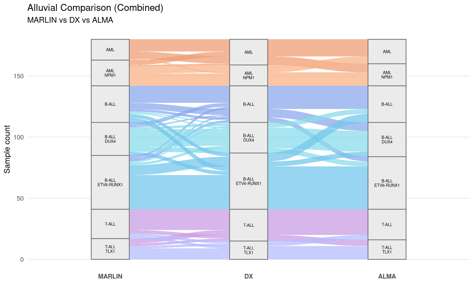
Alluvial Comparison
This script shows how to produce a version of the alluvial comparison panel (MARLIN vs DX vs ALMA), matching the classification-flow view from the full analysis workflow. This code reproduces the base graphic reported in the article Single-workflow Nanopore whole genome sequencing with adaptive sampling for accelerated and comprehensive pediatric cancer profiling.
Overview
The plot compares three aligned classification stages:
MARLINpredicted classDXmolecular diagnosis (reference)ALMApredicted class
Flow width represents sample counts moving through the three stages. This post renders four figures in sequence: combined, ALL-only, AML-only, and a final stacked panel.
Libraries
library(dplyr)
##
## Attaching package: 'dplyr'
## The following objects are masked from 'package:stats':
##
##     filter, lag
## The following objects are masked from 'package:base':
##
##     intersect, setdiff, setequal, union
library(ggplot2)
library(ggalluvial)
library(patchwork)
Define variables
`%nin%` <- Negate(`%in%`)

lineage_from_label <- function(x) {
  ifelse(
    grepl("^B-ALL", x), "B-ALL",
    ifelse(grepl("^T-ALL", x), "T-ALL", "AML")
  )
}

pick_alt_within_lineage <- function(current_label, all_levels) {
  current_lineage <- lineage_from_label(current_label)
  same_lineage_levels <- all_levels[lineage_from_label(all_levels) == current_lineage]
  candidate_levels <- same_lineage_levels[same_lineage_levels != current_label]
  if (length(candidate_levels) == 0) {
    current_label
  } else {
    sample(candidate_levels, 1)
  }
}

lineageCols <- c(
  "B-ALL" = "#8caaee",
  "T-ALL" = "#ca9ee6",
  "AML" = "#ef9f76"
)

metClassColors <- c(
  "B-ALL" = "#8caaee",
  "T-ALL" = "#ca9ee6",
  "AML" = "#ef9f76",
  "B-ALL::ETV6-RUNX1" = "#74c7ec",
  "B-ALL::DUX4" = "#89dceb",
  "T-ALL::TLX1" = "#b4befe",
  "AML::NPM1" = "#fab387"
)
Produce simple test data
set.seed(2026)

n_samples <- 180

dx_levels <- c(
  "B-ALL",
  "T-ALL",
  "AML",
  "B-ALL::ETV6-RUNX1",
  "B-ALL::DUX4",
  "T-ALL::TLX1",
  "AML::NPM1"
)

dx_weights <- c(
  0.18,
  0.14,
  0.12,
  0.20,
  0.14,
  0.10,
  0.12
)

dx_df <- tibble(
  sample_id = sprintf(
    "S%03d",
    seq_len(n_samples)
  ),
  Molecular.Diagnosis = sample(
    dx_levels,
    n_samples,
    replace = TRUE,
    prob = dx_weights
  )
) %>%
  mutate(
    Diagnosis = case_when(
      grepl("^B-ALL", Molecular.Diagnosis) ~
        "B-ALL",
      grepl("^T-ALL", Molecular.Diagnosis) ~
        "T-ALL",
      TRUE ~ "AML"
    )
  )

# Simulate MARLIN and ALMA predictions from DX labels.
# `runif` thresholds control concordance with DX
# (MARLIN ~78%, ALMA ~72%) and introduce off-label noise.
allLeukData <- dx_df %>%
  rowwise() %>%
  mutate(
    mcf = ifelse(
      runif(1) < 0.78,
      Molecular.Diagnosis,
      pick_alt_within_lineage(
        Molecular.Diagnosis,
        dx_levels
      )
    ),
    ALMA.v0.1.14 = ifelse(
      runif(1) < 0.72,
      Molecular.Diagnosis,
      pick_alt_within_lineage(
        Molecular.Diagnosis,
        dx_levels
      )
    ),
    lineage = case_when(
      grepl("^B-ALL", mcf) ~ "B-ALL",
      grepl("^T-ALL", mcf) ~ "T-ALL",
      TRUE ~ "AML"
    ),
    ALMA.Lineage = case_when(
      grepl("^B-ALL", ALMA.v0.1.14) ~
        "B-ALL",
      grepl("^T-ALL", ALMA.v0.1.14) ~
        "T-ALL",
      TRUE ~ "AML"
    )
  ) %>%
  ungroup() %>%
  mutate(
    match.Class = ifelse(
      mcf == Molecular.Diagnosis,
      "TRUE",
      "FALSE"
    ),
    ALMA.match.class = ifelse(
      ALMA.v0.1.14 == Molecular.Diagnosis,
      "TRUE",
      "FALSE"
    )
  )

head(allLeukData)
## # A tibble: 6 × 9
##   sample_id Molecular.Diagnosis Diagnosis mcf         ALMA.v0.1.14      lineage
##   <chr>     <chr>               <chr>     <chr>       <chr>             <chr>
## 1 S001      AML                 AML       AML         AML               AML
## 2 S002      B-ALL::DUX4         B-ALL     B-ALL::DUX4 B-ALL::DUX4       B-ALL
## 3 S003      B-ALL::ETV6-RUNX1   B-ALL     B-ALL       B-ALL::ETV6-RUNX1 B-ALL
## 4 S004      B-ALL               B-ALL     B-ALL       B-ALL             B-ALL
## 5 S005      B-ALL::DUX4         B-ALL     B-ALL::DUX4 B-ALL::DUX4       B-ALL
## 6 S006      B-ALL::ETV6-RUNX1   B-ALL     B-ALL::DUX4 B-ALL::ETV6-RUNX1 B-ALL
## # ℹ 3 more variables: ALMA.Lineage <chr>, match.Class <chr>,
## #   ALMA.match.class <chr>
Build diagnosis subset plots
ALLDataOnly <- allLeukData %>%
  filter(Diagnosis %in% c("B-ALL", "T-ALL"))

p_all_only <- ggplot(
  data = ALLDataOnly,
  aes(
    axis1 = mcf,
    axis2 = Molecular.Diagnosis,
    axis3 = ALMA.v0.1.14
  )
) +
  scale_x_discrete(
    limits = c("MARLIN", "DX", "ALMA")
  ) +
  geom_alluvium(
    aes(fill = Molecular.Diagnosis),
    alpha = 0.8,
    width = 0.275,
    discern = TRUE
  ) +
  geom_stratum(
    width = 0.275,
    fill = "grey95",
    color = "grey40",
    discern = TRUE
  ) +
  geom_text(
    stat = "stratum",
    aes(label = after_stat(ifelse(
      is.na(stratum) | trimws(stratum) == "",
      NA_character_,
      gsub("::", "\n", stratum, fixed = TRUE)
    ))),
    size = 2.1,
    lineheight = 0.9,
    min.y = 2,
    na.rm = TRUE
  ) +
  scale_fill_manual(values = metClassColors) +
  labs(
    title = "ALL-only alluvial",
    x = NULL,
    y = "Sample count"
  ) +
  theme_minimal(base_size = 11) +
  theme(
    legend.position = "none",
    panel.grid.major.x = element_blank()
  )

AMLDataOnly <- allLeukData %>%
  filter(Diagnosis == "AML")

p_aml_only <- ggplot(
  data = AMLDataOnly,
  aes(
    axis1 = mcf,
    axis2 = Molecular.Diagnosis,
    axis3 = ALMA.v0.1.14
  )
) +
  scale_x_discrete(
    limits = c("MARLIN", "DX", "ALMA")
  ) +
  geom_alluvium(
    aes(fill = Molecular.Diagnosis),
    alpha = 0.8,
    width = 0.275,
    discern = TRUE
  ) +
  geom_stratum(
    width = 0.275,
    fill = "grey95",
    color = "grey40",
    discern = TRUE
  ) +
  geom_text(
    stat = "stratum",
    aes(label = after_stat(ifelse(
      is.na(stratum) | trimws(stratum) == "",
      NA_character_,
      gsub("::", "\n", stratum, fixed = TRUE)
    ))),
    size = 2.1,
    lineheight = 0.9,
    min.y = 2,
    na.rm = TRUE
  ) +
  scale_fill_manual(values = metClassColors) +
  labs(
    title = "AML-only alluvial",
    x = NULL,
    y = "Sample count"
  ) +
  theme_minimal(base_size = 11) +
  theme(
    legend.position = "none",
    panel.grid.major.x = element_blank()
  )
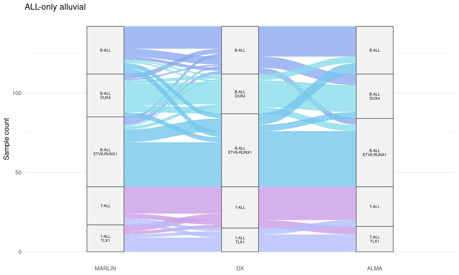
ALL-only plot
p_all_only
## Warning in to_lodes_form(data = data, axes = axis_ind, discern =
## params$discern): Some strata appear at multiple axes.
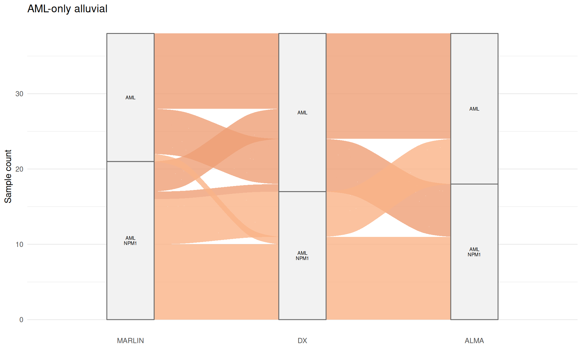
AML-only plot
p_aml_only
## Warning in to_lodes_form(data = data, axes = axis_ind, discern =
## params$discern): Some strata appear at multiple axes.
Main alluvial plot (combined)
p_main <- ggplot(
  data = allLeukData,
  aes(
    axis1 = mcf,
    axis2 = Molecular.Diagnosis,
    axis3 = ALMA.v0.1.14
  )
) +
  scale_x_discrete(
    limits = c("MARLIN", "DX", "ALMA")
  ) +
  geom_alluvium(
    aes(fill = Molecular.Diagnosis),
    alpha = 0.75,
    width = 0.275,
    discern = TRUE
  ) +
  geom_stratum(
    width = 0.275,
    fill = "grey92",
    color = "grey40",
    discern = TRUE
  ) +
  geom_text(
    stat = "stratum",
    aes(label = after_stat(ifelse(
      is.na(stratum) | trimws(stratum) == "",
      NA_character_,
      gsub("::", "\n", stratum, fixed = TRUE)
    ))),
    size = 2.2,
    lineheight = 0.9,
    min.y = 3,
    na.rm = TRUE
  ) +
  scale_fill_manual(
    values = metClassColors
  ) +
  labs(
    title = "Alluvial Comparison (Combined)",
    subtitle = "MARLIN vs DX vs ALMA",
    x = NULL,
    y = "Sample count"
  ) +
  theme_minimal(base_size = 12) +
  theme(
    legend.position = "none",
    panel.grid.major.x = element_blank(),
    panel.grid.minor = element_blank(),
    axis.text.x = element_text(face = "bold")
  )

p_main
## Warning in to_lodes_form(data = data, axes = axis_ind, discern =
## params$discern): Some strata appear at multiple axes.
Save combined plot image
# Export the plot
ggsave(
  filename = "alluvial_comparison_test.png",
  plot = p_main,
  width = 10,
  height = 12,
  dpi = 150
)
## Warning in to_lodes_form(data = data, axes = axis_ind, discern =
## params$discern): Some strata appear at multiple axes.
Session Info
## R version 4.5.2 (2025-10-31)
## Platform: x86_64-pc-linux-gnu
## Running under: Linux Mint 22.2
##
## Matrix products: default
## BLAS:   /usr/lib/x86_64-linux-gnu/blas/libblas.so.3.12.0
## LAPACK: /usr/lib/x86_64-linux-gnu/lapack/liblapack.so.3.12.0  LAPACK version 3.12.0
##
## locale:
##  [1] LC_CTYPE=en_CA.UTF-8       LC_NUMERIC=C
##  [3] LC_TIME=en_CA.UTF-8        LC_COLLATE=en_CA.UTF-8
##  [5] LC_MONETARY=en_CA.UTF-8    LC_MESSAGES=en_CA.UTF-8
##  [7] LC_PAPER=en_CA.UTF-8       LC_NAME=C
##  [9] LC_ADDRESS=C               LC_TELEPHONE=C
## [11] LC_MEASUREMENT=en_CA.UTF-8 LC_IDENTIFICATION=C
##
## time zone: America/Toronto
## tzcode source: system (glibc)
##
## attached base packages:
## [1] stats     graphics  grDevices utils     datasets  methods   base
##
## other attached packages:
## [1] patchwork_1.3.2   ggalluvial_0.12.6 ggplot2_4.0.2     dplyr_1.2.0
##
## loaded via a namespace (and not attached):
##  [1] gtable_0.3.6       jsonlite_2.0.0     compiler_4.5.2     tidyselect_1.2.1
##  [5] tidyr_1.3.2        jquerylib_0.1.4    scales_1.4.0       yaml_2.3.12
##  [9] fastmap_1.2.0      R6_2.6.1           labeling_0.4.3     generics_0.1.4
## [13] knitr_1.51         tibble_3.3.1       bookdown_0.46      bslib_0.10.0
## [17] pillar_1.11.1      RColorBrewer_1.1-3 rlang_1.1.7        utf8_1.2.6
## [21] cachem_1.1.0       xfun_0.56          sass_0.4.10        S7_0.2.1
## [25] otel_0.2.0         cli_3.6.5          withr_3.0.2        magrittr_2.0.4
## [29] digest_0.6.39      grid_4.5.2         lifecycle_1.0.5    vctrs_0.7.1
## [33] evaluate_1.0.5     glue_1.8.0         farver_2.1.2       blogdown_1.23
## [37] purrr_1.2.1        rmarkdown_2.30     tools_4.5.2        pkgconfig_2.0.3
## [41] htmltools_0.5.9
